Data
For a class exercise, a hypothetical data set was created based on a partial data set from the actual 2013 field study. The interpretation of this data should be regarded as fictional.
A subset of the hypothetical data set is provided in Table 2. The predictor variables of most importance in determining the optimal lure are "Volatiles","Dose", and "TubeSize". "Site" is included to block for variation between farms. I am also interested in understanding the phenology of the pea leaf weevil, so "Week" and "Season" were also included. The responding variable ("Capture") is the number of pea leaf weevils found in each trap, each week. Similarly, the experimental unit in this study is the number of pea leaf weevils in each trap.
A subset of the hypothetical data set is provided in Table 2. The predictor variables of most importance in determining the optimal lure are "Volatiles","Dose", and "TubeSize". "Site" is included to block for variation between farms. I am also interested in understanding the phenology of the pea leaf weevil, so "Week" and "Season" were also included. The responding variable ("Capture") is the number of pea leaf weevils found in each trap, each week. Similarly, the experimental unit in this study is the number of pea leaf weevils in each trap.
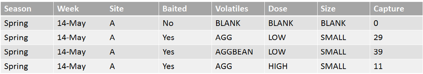
Table 2. Sample data for the experiment testing the attractiveness of eight traps baited with aggregation pheromones and host plant volatiles and one blank to adult pea leaf weevils.
The analysis of this study was performed separately for the spring and fall trapping periods. To show that baited traps were significantly more attractive than blank traps, I used a Wilcox rank sum test. To determine the most attractive lure, I analyzed my data in R with a mixed effects model:
lmer(sqrt_Captures~Volatiles+Dose+TubeSize+(1|Site))
A square root transformation of the dependent variable "Captures" was included to meet the assumptions of normality (Figure 10). With this square root transformation included, the data in the models is normally distributed for both the spring and fall. The residuals for this model are also normally distributed and evenly dispersed. Other models testing other transformations and including interaction effects were also developed, but these models did not have the best fit for my data. No significant interactions were found.
To gain a further understanding of pea leaf weevil phenology, the weekly capture of pea leaf weevils in an optimally baited trap was visually inspected for the spring and fall flight periods.
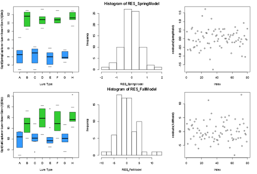
Figure 12. The data meets the assumptions for the mixed effects model. Data for the spring is represented in the top three graphs and for the fall in the bottom three. Boxplots show that within each lure type, the data is normally distributed under this model (left). The residuals of this model are normally distributed (center) and evenly dispersed (right).
